
The following is a lightly edited version of the contents of an email by reader Rob Maurer. He’s an Associate Professor of Health Systems Management at Texas Woman’s University. In addition to nearly all the words, the charts are his.
I looked at the Hoenig & Heisey and the Goodman & Berlin papers that Austin cited. I suspect that the difference between what they discuss and what he and colleagues did might be more clearly expressed in charts.
The essence of Goodman & Berlin’s argument is the following (p. 202)
The power of an experiment is the pretrial probability of all nonsignificant outcomes taken together (under a specified alternative hypothesis), and any attempt to apply power to a single outcome is problematic. When people try to use power in that way, they immediately encounter the problem that there is not a unique power estimate to use; there is a different power for each underlying difference.
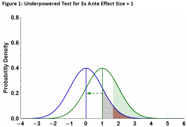
To illustrate, start with an ex ante power calculation as depicted in Figure 1. The blue curve is the null distribution (e.g., no Medicaid) and the green curve is the distribution for effect size = 1 (e.g., with Medicaid). The shaded red(ish) area is the type 1 error rate (5%), the shaded green area is the test power, and the black striped area is the p-value for observed effect size = 1 (which results in a failure to reject the null since it is larger than 5%). Clearly, every choice of ex ante effect produces a different test power.
As for post-experiment (or post hoc) power, Goodman & Berlin then comment (p. 202):
To eliminate this ambiguity, some researchers calculate the power with respect to the observed difference, a number that is at least unique. This is what is called the “post hoc power.” … The unstated rationale for the calculation is roughly as follows: It is usually done when the researcher believes there is a treatment difference, despite the nonsignificant result.
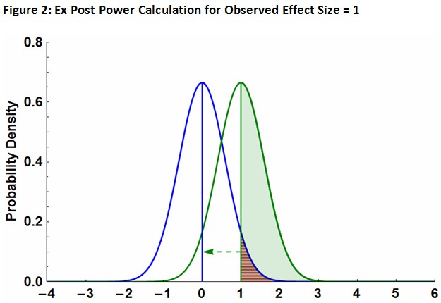
In my example, the post hoc power calculation for an observed effect size = 1 is depicted in Figure 2. The fact that we need a smaller standard error to increase the power (to a 5% type 1 error threshold) implies that we need a larger sample. Note that this is equivalent to saying that the p-value and the type 1 error rate, in this case, have the same value.
Goodman & Berlin go on to observe (p. 202):
The notion of the P value as an “observed” type I error suffers from the same logical problems as post hoc power. Once we know the observed result, the notion of an “error rate” is no longer meaningful in the same way that it was before the experiment.
This comment, identifying a post hoc power calculation with the mistake of identifying the p-value with an observed type 1 error rate, makes clear what Goodman & Berlin have in mind when they say “power should play no role once the data have been collected.” Figure 2 shows how the two are related.
What I think Austin et al. are doing with their power calculations is depicted in Figure 3 (which is identical to Figure 1 except effect size = 2). I labeled the figure as a post hoc calculation of the ex ante test power to emphasize that, yes, it is after-the-fact but is focused on ex ante power. What this shows is that, given the existing sample size, one needs a large effect to have sufficient power to reject a false null.
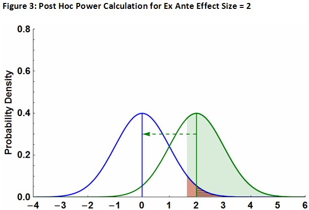
Where I think the discussion in comments to posts on this blog about this subject has gone off track is that “larger effect size” and “larger sample size” get confused. Goodman & Berlin are arguing against a post hoc justification for a larger sample size (Figure 2) where I think Austin et al. are arguing that a larger ex ante effect is required to justify a failure to reject the null given the sample size used in the study (Figure 3).
One can make the same point by saying that the study did not have sufficient ex ante power (which could have been addressed by increasing the sample size), but that is not the same as a post hoc power calculation.
I think what Austin et al.’s argument boils down to is that, given the small sample size and resulting standard error, there is a range of small effect sizes that produce an ambiguous result. The ex ante effect size they obtained from the literature can be interpreted to suggest that the observed effect falls in this ambiguous range, hence the need for more power.