
Sorry for the false start last night. More about that here. I still welcome comments if you find any errors.
This is a follow up to my several prior posts on how to adjust a power calculation to account for an instrumental variable (IV) design. The details are in a new PDF. (If you downloaded the one I posted last night, replace it with this one.) First, for the non-geeks:
- Skip the proof and jump to the example that begins on page two of the PDF. It runs through the numbers for the Medicaid study result for glycated hemoglobin (GH), which I had used to illustrate the power issues in my first post on this topic. (It’s a commentary on this blog’s readership that I can even consider this example suitable for non-geeks. I guess I mean geeks of a different order.)
- One thing you may notice is that the Medicaid and non-Medicaid groups are different sizes than you might have expected if you only read the paper and not the appendix. I refer you to appendix table S9 for the details. Suffice it to say, it is not true that 24.1% of the lottery winners took up Medicaid. There were a lot more Medicaid enrollees than that. (What is true is that 24.1% more lottery winners took up Medicaid than non-winners.)
- For that reason, and because I was targeting 95% power, my estimate in my first post was quite a bit off. I thought the study was underpowered by a factor of 5 for the GH measure. Actually, according to the methods in that post, and using the new numbers and targeting 80% power (which, I am told, is more standard), the study is only underpowered by a factor of 1.5.
- But, as I wrote in that post, I had not accounted for the IV design. The new calculation does so. And that, my friends, really wallops power and precision. The bottom line is, accounting for the design, the GH analysis was underpowered by about a factor of 23 (yes, twenty-three!) meaning it’d have needed that multiple of sample to be able to detect a true Medicaid effect with 80% probability.
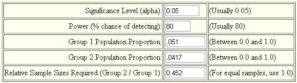
- You can run the numbers for other measures using this online tool. The underpowering will vary. Below is a screenshot for the inputs for the GH analysis. Follow the steps in the PDF for the rest. (Hint: multiply the sample sizes from the online tool by 14.8.)
Now, for the uber-geeks, the content of the PDF differs from my prior version of a few days ago in three ways:
- It properly accounts for the fact that we were assuming all vectors were zero mean. That didn’t affect the result, but it does affect how you should simulate the first stage (which we’ve done for you for the Medicaid study in the document).
- It references Wooldridge, who obtained the same result. (So, we’re right!)
- It includes a complete example from the Medicaid study. However, don’t overlook the fact that this generalizes. Truth be told, I didn’t do all this to comment on the Medicaid study. I need this for my own work.
I should point out that the finding that the variance of the effect size in an RCT scales with the inverse of Np(1-p) is beautiful. It doesn’t just scale with 1/N because it is the mean of a difference. When p goes to zero, there are no treatments. When p goes to 1, there are no controls. Either way, the variance of the difference in effect size has to go to infinity. And, indeed it does. This is comforting intuition.
Finally, I’m grateful for the awesome feedback I’ve received from readers. Once again, the TIE community has hit this one out of the park. Thank you.